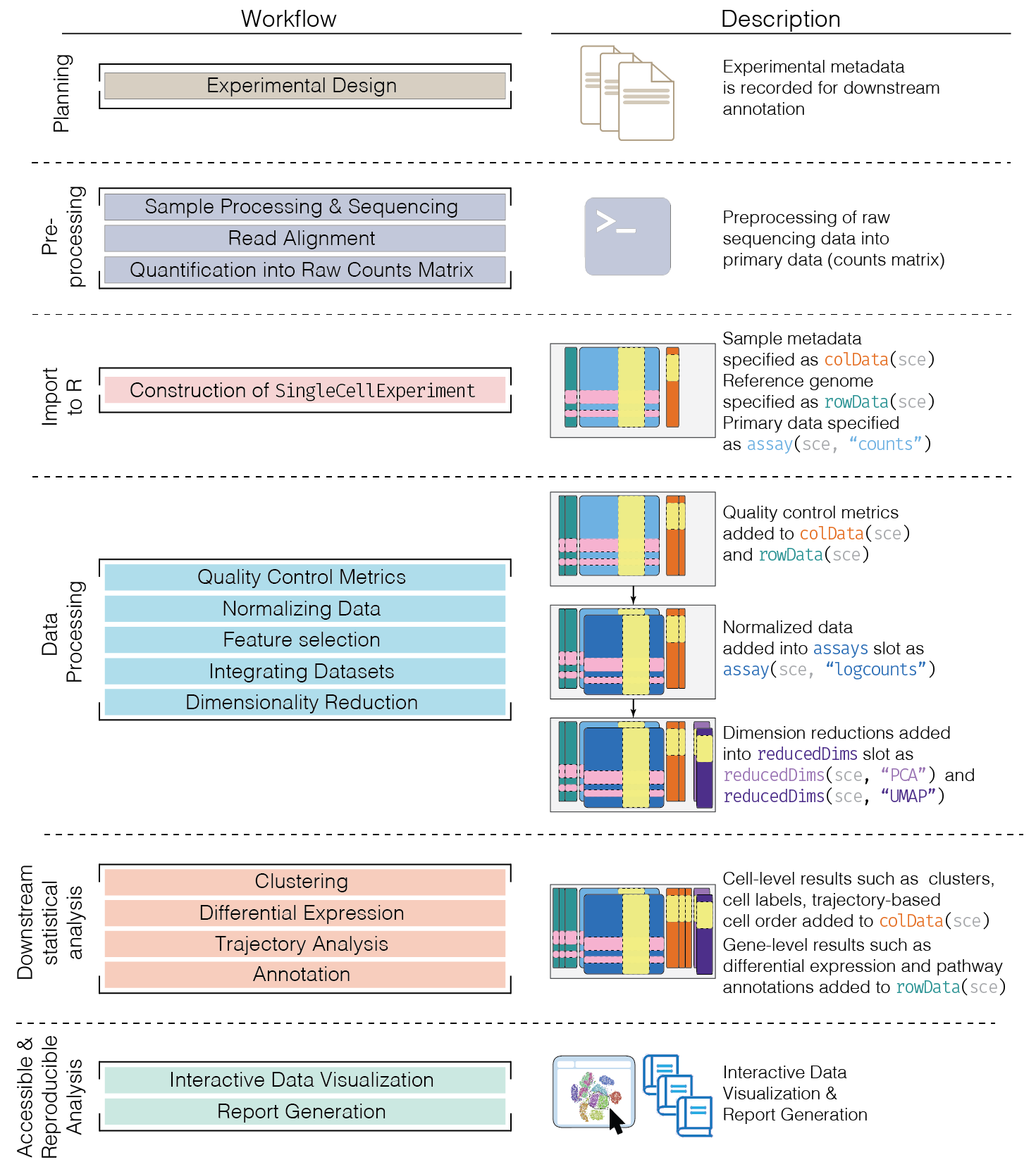
Seurat is very high integrated package. Actually, the basic workflow of scRNA-seq analysis is:

1. We compute quality control metrics to remove low-quality cells that would interfere with downstream analyses. These cells may have been damaged during processing or may not have been fully captured by the sequencing protocol. Common metrics includes the total counts per cell, the proportion of spike-in or mitochondrial reads and the number of detected features.
2. We convert the counts into normalized expression values to eliminate cell-specific biases (e.g., in capture efficiency). This allows us to perform explicit comparisons across cells in downstream steps like clustering. We also apply a transformation, typically log, to adjust for the mean-variance relationship.
3. We perform feature selection to pick a subset of interesting features for downstream analysis. This is done by modelling the variance across cells for each gene and retaining genes that are highly variable. The aim is to reduce computational overhead and noise from uninteresting genes.
4. We apply dimensionality reduction to compact the data and further reduce noise. Principal components analysis is typically used to obtain an initial low-rank representation for more computational work, followed by more aggressive methods like tstochastic neighbor embedding for visualization purposes.
5. We cluster cells into groups according to similarities in their (normalized) expression profiles. This aims to obtain groupings that serve as empirical proxies for distinct biological states. We typically interpret these groupings by identifying differentially expressed marker genes between clusters.

Test code

Example code from here

library(scRNAseq)

sce.zeisel <- ZeiselBrainData()

library(scater)

library(BiocFileCache)
bfc <- BiocFileCache(ask=FALSE)
url <- file.path("ftp://ftp.ncbi.nlm.nih.gov/geo/series",
    "GSE85nnn/GSE85241/suppl",
    "GSE85241%5Fcellsystems%5Fdataset%5F4donors%5Fupdated%2Ecsv%2Egz")
muraro.fname <- bfcrpath(bfc, url)
local.name <- URLdecode(basename(url))
unlink(local.name)
if (.Platform$OS.type=="windows") {
    file.copy(muraro.fname, local.name)
} else {
    file.symlink(muraro.fname, local.name)
}

mat <- as.matrix(read.delim("GSE85241_cellsystems_dataset_4donors_updated.csv.gz"))

dim(mat)
mat[1:4,1:4]
class(mat)
object.size(mat)

library(scuttle)
sparse.mat <- readSparseCounts(local.name)

dim(sparse.mat)
sparse.mat[1:4,1:4]
class(sparse.mat)
object.size(sparse.mat)

library(DropletUtils)
sce <- read10xCounts("/home/liuc9/tmp/singlecell/filtered_gene_bc_matrices/hg19")

sce

SingleCellExperiment class

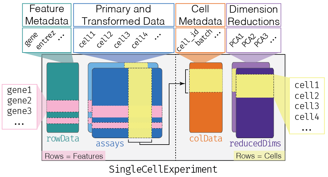
sce@colData
sce@metadata

barcodes <- readr::read_tsv(file = "/home/liuc9/tmp/singlecell/filtered_gene_bc_matrices/hg19/barcodes.tsv", col_names = FALSE)
features <- readr::read_tsv(file = "/home/liuc9/tmp/singlecell/filtered_gene_bc_matrices/hg19/genes.tsv", col_names = FALSE)
mtx <- Matrix::readMM(file = "/home/liuc9/tmp/singlecell/filtered_gene_bc_matrices/hg19/matrix.mtx")
rownames(mtx) <- features$X1
colnames(mtx) <- barcodes$X1

sce <- SingleCellExperiment(
  assays = list(counts = mtx)
)

sce <- scuttle::logNormCounts(sce)

counts_100 <- counts(sce) + 100
assay(sce, "counts_100") <- counts_100
# assay(sce)
sce

assays(sce) <- assays(sce)[1:2]

sce

assayNames(sce)

Dimensionality reduction

library(DropletUtils)
sce <- read10xCounts("/home/liuc9/tmp/singlecell/filtered_gene_bc_matrices/hg19")

sce %>%
  scater::logNormCounts() %>%
  scater::runPCA() ->
  sce

sce

reducedDim(sce, "PCA") %>% dim()

sce <- scater::runTSNE(sce, perplexity = 0.1)

head(reducedDim(sce, "TSNE"))

sce

reducedDim(sce, "TSNE") %>% head()

reducedDims(sce)

u <- uwot::umap(t(logcounts(sce)), n_neighbors = 2)

sce <- scater::runUMAP(sce)

reducedDims(sce)

size factor

sce <- scran::computeSumFactors(sce)

sce

colLabels(sce) <-  scran::clusterCells(sce, use.dimred = "PCA")

colLabels(sce) %>% table

Analysis overview

sce <- scRNAseq::MacoskoRetinaData()

sce

is.mito <- grepl("^MT-", rownames(sce))
qcstats <- scater::perCellQCMetrics(sce, subset = list(Mito = is.mito))
filtered <- scater::quickPerCellQC(qcstats, percent_subsets="subsets_Mito_percent")

sce <- sce[, !filtered$discard]

sce

sce <- scater::logNormCounts(sce)

sce
sce@colData %>% head()

dec <- scran::modelGeneVar(sce)
hvg <- scran::getTopHVGs(dec, prop = 0.1)

dec

set.seed(1234)

sce <- scater::runPCA(sce, ncomponents=25, subset_row=hvg)

sce

colLabels(sce) <- scran::clusterCells(
  x = sce,
  use.dimred = "PCA",
  BLUSPARAM = bluster::NNGraphParam(
    cluster.fun = "louvain"
  )
)

sce$label %>% table()

sce <- scater::runUMAP(sce, dimred="PCA")

sce

reducedDim(sce, "UMAP") %>% head()

scater::plotUMAP(sce, colour_by = "label")

# Marker detection.
markers <- scran::findMarkers(sce, test.type="wilcox", direction="up", lfc=1)

dim(sce)
sce$label %>% table()
markers$`1` %>% dim()
markers$`1`

Multiple batches

sce <- scRNAseq::SegerstolpePancreasData()

qcstats <- scater::perCellQCMetrics(sce)
filtered <- scater::quickPerCellQC(qcstats, percent_subsets="altexps_ERCC_percent")
sce <- sce[, !filtered$discard]

sce <- scater::logNormCounts(sce)

dec <- scran::modelGeneVar(sce, block=sce$individual)
hvg <- scran::getTopHVGs(dec, prop = 0.1)

dec %>% dim()

set.seed(1234)

sce <- batchelor::correctExperiments(
  sce,
  batch=sce$individual,
  subset.row=hvg,
  correct.all=TRUE
)

colLabels(sce) <- scran::clusterCells(sce, use.dimred='corrected')

sce <- scater::runUMAP(sce, dimred="corrected")

sce

gridExtra::grid.arrange(
    scater::plotUMAP(sce, colour_by="label"),
    scater::plotUMAP(sce, colour_by="individual"),
    ncol=2
)

# Marker detection, blocking on the individual of origin.
markers <- scran::findMarkers(sce, test.type="wilcox", direction="up", lfc=1)